Key Features
Eager search spaces
Automated search for optimal hyperparameters using Python conditionals, loops, and syntax
State-of-the-art algorithms
Efficiently search large spaces and prune unpromising trials for faster results
Easy parallelization

Parallelize hyperparameter searches over multiple threads or processes without modifying code
Code Examples
Optuna is framework agnostic. You can use it with any machine learning or deep learning framework.
A simple optimization problem:
- Define
objectivefunction to be optimized. Let's minimize(x - 2)^2 - Suggest hyperparameter values using
trialobject. Here, a float value ofxis suggested from-10to10 - Create a
studyobject and invoke theoptimizemethod over 100 trials
import optuna

def objective(trial):
    x = trial.suggest_float('x', -10, 10)
    return (x - 2) ** 2

study = optuna.create_study()
study.optimize(objective, n_trials=100)

study.best_params # E.g. {'x': 2.002108042}You can optimize PyTorch hyperparameters, such as the number of layers and the number of hidden nodes in each layer, in three steps:
- Wrap model training with an
objectivefunction and return accuracy - Suggest hyperparameters using a
trialobject - Create a
studyobject and execute the optimization
import torch

import optuna

# 1. Define an objective function to be maximized.
def objective(trial):

    # 2. Suggest values of the hyperparameters using a trial object.
    n_layers = trial.suggest_int('n_layers', 1, 3)
    layers = []

    in_features = 28 * 28
    for i in range(n_layers):
        out_features = trial.suggest_int(f'n_units_l{i}', 4, 128)
        layers.append(torch.nn.Linear(in_features, out_features))
        layers.append(torch.nn.ReLU())
        in_features = out_features
    layers.append(torch.nn.Linear(in_features, 10))
    layers.append(torch.nn.LogSoftmax(dim=1))
    model = torch.nn.Sequential(*layers).to(torch.device('cpu'))
    ...
    return accuracy

# 3. Create a study object and optimize the objective function.
study = optuna.create_study(direction='maximize')
study.optimize(objective, n_trials=100)You can optimize TensorFlow hyperparameters, such as the number of layers and the number of hidden nodes in each layer, in three steps:
- Wrap model training with an
objectivefunction and return accuracy - Suggest hyperparameters using a
trialobject - Create a
studyobject and execute the optimization
import tensorflow as tf

import optuna

# 1. Define an objective function to be maximized.
def objective(trial):

    # 2. Suggest values of the hyperparameters using a trial object.
    n_layers = trial.suggest_int('n_layers', 1, 3)
    model = tf.keras.Sequential()
    model.add(tf.keras.layers.Flatten())
    for i in range(n_layers):
        num_hidden = trial.suggest_int(f'n_units_l{i}', 4, 128, log=True)
        model.add(tf.keras.layers.Dense(num_hidden, activation='relu'))
    model.add(tf.keras.layers.Dense(CLASSES))
    ...
    return accuracy

# 3. Create a study object and optimize the objective function.
study = optuna.create_study(direction='maximize')
study.optimize(objective, n_trials=100)You can optimize Keras hyperparameters, such as the number of filters and kernel size, in three steps:
- Wrap model training with an
objectivefunction and return accuracy - Suggest hyperparameters using a
trialobject - Create a
studyobject and execute the optimization
import keras

import optuna

# 1. Define an objective function to be maximized.
def objective(trial):
    model = Sequential()

    # 2. Suggest values of the hyperparameters using a trial object.
    model.add(
        Conv2D(filters=trial.suggest_categorical('filters', [32, 64]),
               kernel_size=trial.suggest_categorical('kernel_size', [3, 5]),
               strides=trial.suggest_categorical('strides', [1, 2]),
               activation=trial.suggest_categorical('activation', ['relu', 'linear']),
               input_shape=input_shape))
    model.add(Flatten())
    model.add(Dense(CLASSES, activation='softmax'))

    # We compile our model with a sampled learning rate.
    lr = trial.suggest_float('lr', 1e-5, 1e-1, log=True)
    model.compile(loss='sparse_categorical_crossentropy', optimizer=RMSprop(lr=lr), metrics=['accuracy'])
    ...
    return accuracy

# 3. Create a study object and optimize the objective function.
study = optuna.create_study(direction='maximize')
study.optimize(objective, n_trials=100)
You can optimize Scikit-Learn hyperparameters, such as the C parameter of
SVC and the max_depth of the RandomForestClassifier,
in
three steps:
- Wrap model training with an
objectivefunction and return accuracy - Suggest hyperparameters using a
trialobject - Create a
studyobject and execute the optimization
import sklearn

import optuna

# 1. Define an objective function to be maximized.
def objective(trial):

    # 2. Suggest values for the hyperparameters using a trial object.
    classifier_name = trial.suggest_categorical('classifier', ['SVC', 'RandomForest'])
    if classifier_name == 'SVC':
         svc_c = trial.suggest_float('svc_c', 1e-10, 1e10, log=True)
         classifier_obj = sklearn.svm.SVC(C=svc_c, gamma='auto')
    else:
        rf_max_depth = trial.suggest_int('rf_max_depth', 2, 32, log=True)
        classifier_obj = sklearn.ensemble.RandomForestClassifier(max_depth=rf_max_depth, n_estimators=10)
    ...
    return accuracy

# 3. Create a study object and optimize the objective function.
study = optuna.create_study(direction='maximize')
study.optimize(objective, n_trials=100)You can optimize XGBoost hyperparameters, such as the booster type and alpha, in three steps:
- Wrap model training with an
objectivefunction and return accuracy - Suggest hyperparameters using a
trialobject - Create a
studyobject and execute the optimization
import xgboost as xgb

import optuna

# 1. Define an objective function to be maximized.
def objective(trial):
    ...

    # 2. Suggest values of the hyperparameters using a trial object.
    param = {
        "objective": "binary:logistic",
        "booster": trial.suggest_categorical("booster", ["gbtree", "gblinear", "dart"]),
        "lambda": trial.suggest_float("lambda", 1e-8, 1.0, log=True),
        "alpha": trial.suggest_float("alpha", 1e-8, 1.0, log=True),
        "subsample": trial.suggest_float("subsample", 0.2, 1.0),
        "colsample_bytree": trial.suggest_float("colsample_bytree", 0.2, 1.0),
    }

    bst = xgb.train(param, dtrain)
    ...
    return accuracy

# 3. Create a study object and optimize the objective function.
study = optuna.create_study(direction='maximize')
study.optimize(objective, n_trials=100)You can optimize LightGBM hyperparameters, such as boosting type and the number of leaves, in three steps:
- Wrap model training with an
objectivefunction and return accuracy - Suggest hyperparameters using a
trialobject - Create a
studyobject and execute the optimization
import lightgbm as lgb

import optuna

# 1. Define an objective function to be maximized.
def objective(trial):
    ...

    # 2. Suggest values of the hyperparameters using a trial object.
    param = {
        'objective': 'binary',
        'metric': 'binary_logloss',
        'verbosity': -1,
        'boosting_type': 'gbdt',
        'lambda_l1': trial.suggest_float('lambda_l1', 1e-8, 10.0, log=True),
        'lambda_l2': trial.suggest_float('lambda_l2', 1e-8, 10.0, log=True),
        'num_leaves': trial.suggest_int('num_leaves', 2, 256),
        'feature_fraction': trial.suggest_float('feature_fraction', 0.4, 1.0),
        'bagging_fraction': trial.suggest_float('bagging_fraction', 0.4, 1.0),
        'bagging_freq': trial.suggest_int('bagging_freq', 1, 7),
        'min_child_samples': trial.suggest_int('min_child_samples', 5, 100),
    }

    gbm = lgb.train(param, dtrain)
    ...
    return accuracy

# 3. Create a study object and optimize the objective function.
study = optuna.create_study(direction='maximize')
study.optimize(objective, n_trials=100)
Check more examples including PyTorch Ignite, Dask-ML and MLFlow at our GitHub
repository.
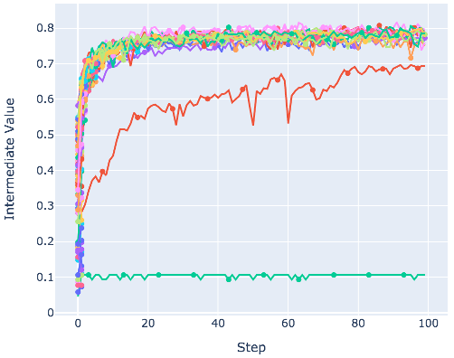
It also provides the visualization demo as follows:
from optuna.visualization import plot_intermediate_values

...
plot_intermediate_values(study)
Installation
Dashboard
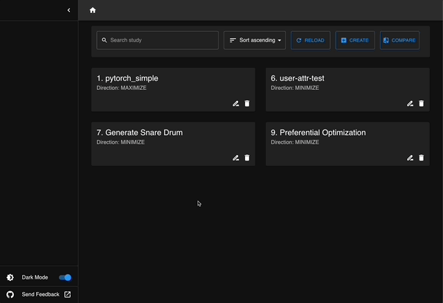
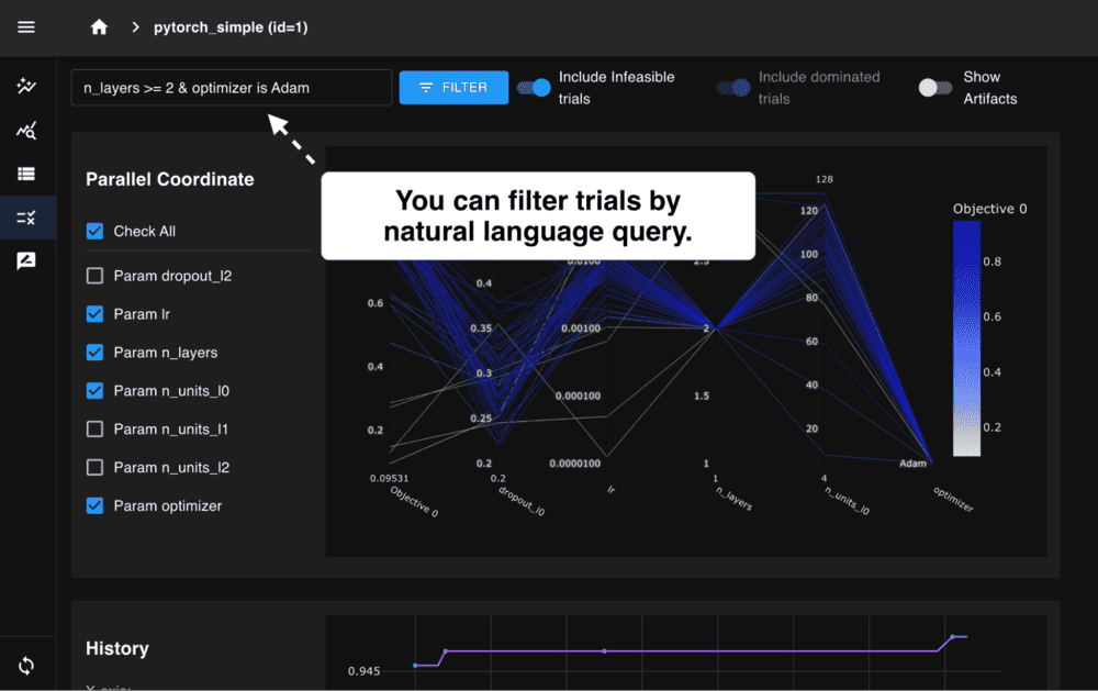
Optuna Dashboard is a real-time web dashboard for Optuna. You can check the optimization history, hyperparameter importances, etc. in graphs and tables.
% pip install optuna-dashboard
% optuna-dashboard sqlite:///db.sqlite3
Optuna Dashboard is also available as extensions for Jupyter Lab and Visual Studio Code.
VS Code Extension
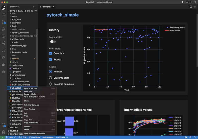
To use, install the extension, right-click the SQLite3 files in the file explorer and select the “Open in Optuna Dashboard” from the dropdown menu.
Jupyter Lab Extension
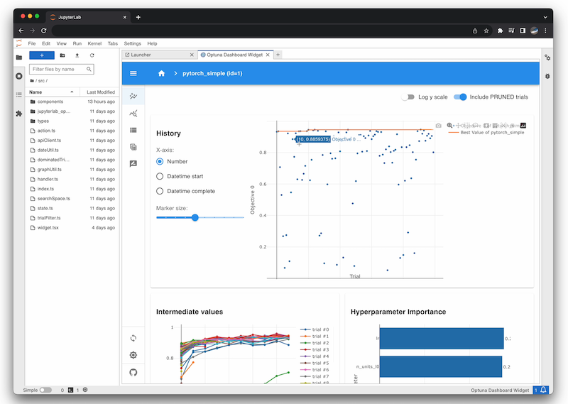
% pip install jupyterlab jupyterlab-optunaOptunaHub
OptunaHub is a feature-sharing platform for Optuna. Users can freely use registered features, and contributors can register the features they implement. The following example uses AutoSampler on OptunaHub, which automatically selects a proper sampler from those implemented in Optuna.
% pip install optunahub
% pip install cmaes scipy torch  # install AutoSampler dependencies
import optuna
import optunahub
def objective(trial: optuna.Trial) -> float:
x = trial.suggest_float("x", -5, 5)
y = trial.suggest_float("y", -5, 5)
return x**2 + y**2
module = optunahub.load_module(package="samplers/auto_sampler")
study = optuna.create_study(sampler=module.AutoSampler())
study.optimize(objective, n_trials=50)
print(study.best_trial.value, study.best_trial.params)Blog
 We are excited to announce the release of Optuna 4.6, the latest version of our black-box optimization framework.
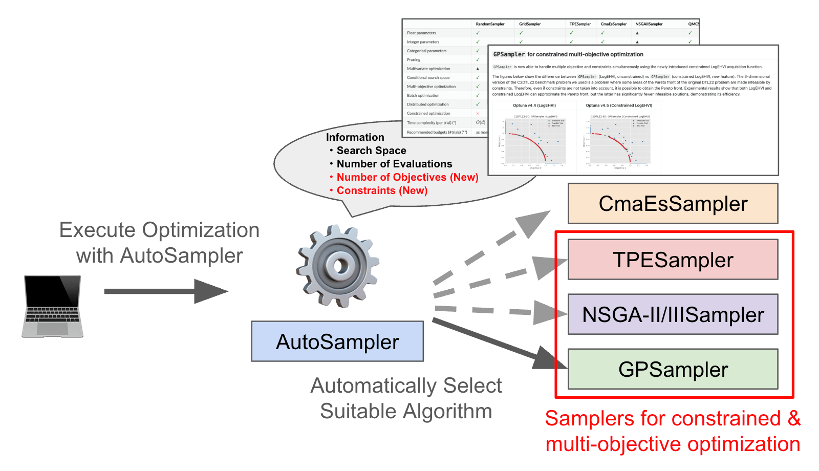 We have enhanced AutoSampler to fully support multi-objective and constrained optimization.
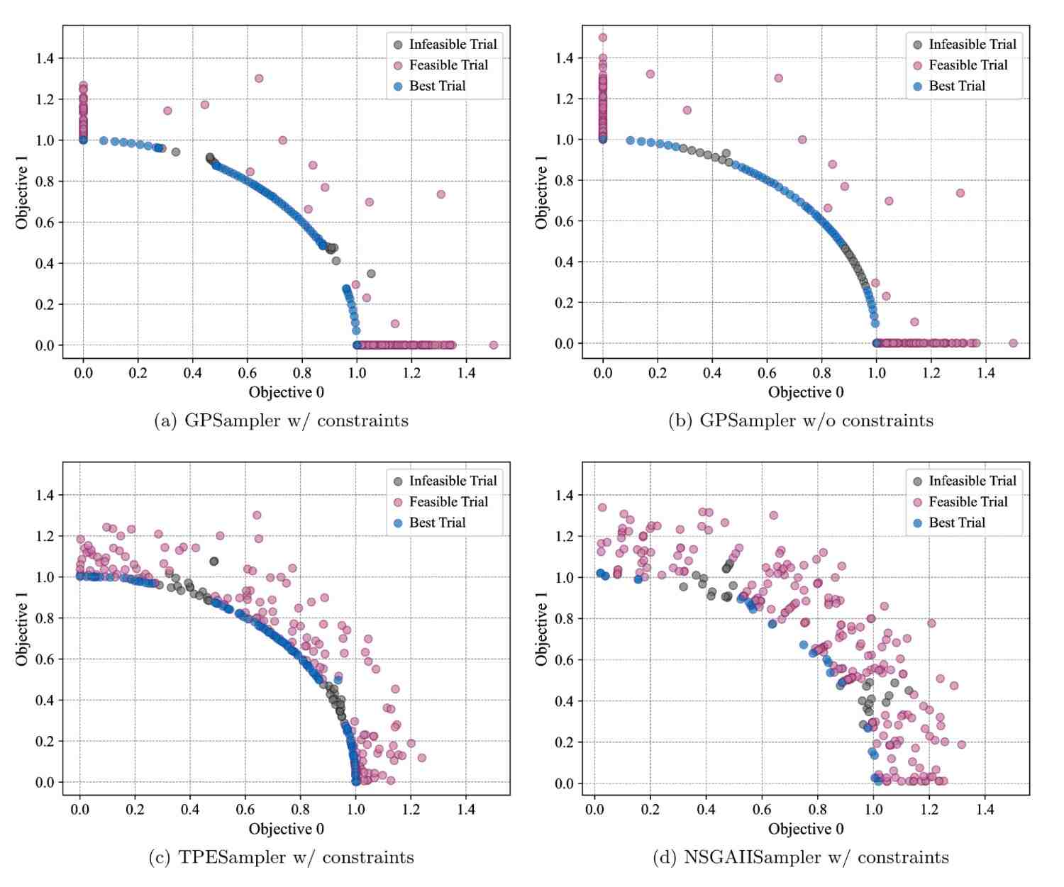 Optuna v4.5 extends Gaussian process-based sampler (GPSampler) to support constrained multi-objective optimization.
 We have released the version 4.4 of the black-box optimization framework Optuna. We encourage you to check out the release notes!
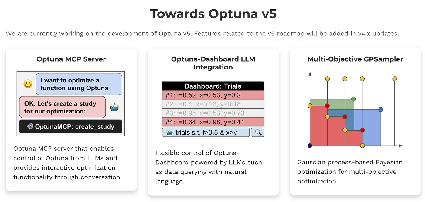 Optuna v5 pushes black-box optimization forward - with new features for generative AI, broader applications, and easier integration.
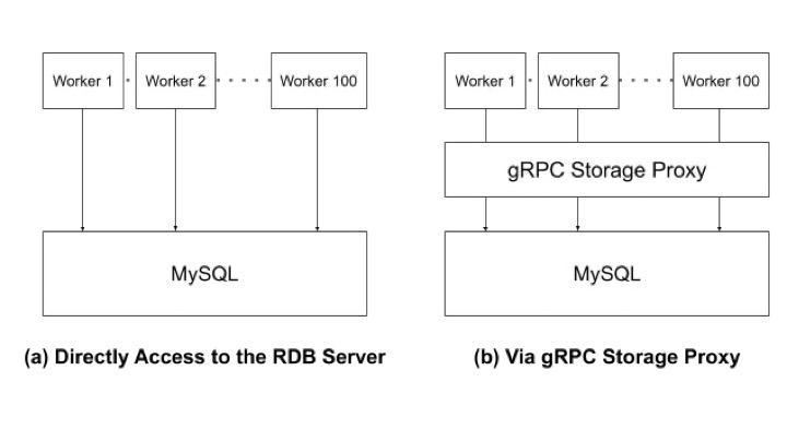 This article explains how to perform distributed optimization and introduce the gRPC Storage Proxy, which enables large-scale optimization.
Videos
Papers
Optuna
If you use Optuna in a scientific publication, please use the following citation:
Takuya Akiba, Shotaro Sano, Toshihiko Yanase, Takeru Ohta, and Masanori Koyama. 2019.
	Optuna: A Next-generation Hyperparameter Optimization Framework. In KDD.
Bibtex entry:
@inproceedings{optuna_2019,
	title={Optuna: A Next-generation Hyperparameter Optimization Framework},
	author={Akiba, Takuya and Sano, Shotaro and Yanase, Toshihiko and Ohta, Takeru and Koyama, Masanori},
	booktitle={Proceedings of the 25th {ACM} {SIGKDD} International Conference on Knowledge Discovery and Data Mining},
	year={2019}
}
View
Paper
arXiv
Preprint
OptunaHub
If you use OptunaHub in a scientific publication, please use the following citation:
Yoshihiko Ozaki, Shuhei Watanabe, and Toshihiko Yanase. 2025.
	OptunaHub: A Platform for Black-Box Optimization. arXiv preprint arXiv:2510.02798.
Bibtex entry:
@article{ozaki2025optunahub,
	title={{OptunaHub}: A Platform for Black-Box Optimization},
	author={Ozaki, Yoshihiko and Watanabe, Shuhei and Yanase, Toshihiko},
	journal={arXiv preprint arXiv:2510.02798},
	year={2025}
}
arXiv
Preprint